 Photo by Safar Safarov on Unsplash
引入
首先,我们随机生成一组数据 \begin{equation}\label{eq:1} y = \sin(x) + \epsilon \\ x \in [1\pi/3,5\pi/3] \end{equation} $\epsilon$是一个随机扰动
import numpy as np
import pandas as pd
import random
import matplotlib.pyplot as plt

%matplotlib inline
from matplotlib.pylab import rcParams

rcParams["figure.figsize"] = 12, 10

x = np.array([i * np.pi / 180 for i in range(60, 300, 4)])
np.random.seed(10)
y = np.sin(x) + np.random.normal(0, 0.15, len(x))
data = pd.DataFrame(np.column_stack([x,y]),columns=['x','y'])
plt.plot(data['x'],data['y'],'.')

因为噪点的存在,数据分布并不完全服从$\sin$曲线。现在,我们准备使用多项式回归去拟合数据分布,我们依次将$x$的1阶到15阶加入到数据中 \begin{equation} \label{eq:2} y = \theta _1 x^1 + ... + \theta _n x^n \\ n = 1,...,15 \end{equation}
for i in range(2, 16):
    colname = "x_%d" % i
    data[colname] = data["x"] ** i
print(data.head())
我们建立15个不同的线性回归模型,第$i$个模型包含从$x^1$到$x^i$变量。例如,第8个模型就包括 $\{x^1, x^2, x^3,…,x^8\}$。
from sklearn.linear_model import LinearRegression


def linear_regression(data, power, models_to_plot):
    r"""returns a list containing – [ model RSS, intercept, coef_x, coef_x2, … upto entered power ].
    ----------
    power : int
        Maximum power of x

    RSS :float
        Sum of square of errors between the predicted and actual values in the training data set

    models_to_plot: dict
        A dict containg the model to be ploted

    Returns
    -------
    list
         [ model RSS, intercept, coef_x, coef_x2, … upto entered power ]

    """
    # initialize predictors:
    predictors = ["x"]
    if power >= 2:
        predictors.extend(["x_%d" % i for i in range(2, power + 1)])

    # Fit the model
    linreg = LinearRegression(normalize=True)
    linreg.fit(data[predictors], data["y"])
    y_pred = linreg.predict(data[predictors])

    # Check if a plot is to be made for the entered power
    if power in models_to_plot:
        plt.subplot(models_to_plot[power])
        plt.tight_layout()
        plt.plot(data["x"], y_pred)
        plt.plot(data["x"], data["y"], ".")
        plt.title("Plot for power: %d" % power)

    # Return the result in pre-defined format
    rss = sum((y_pred - data["y"]) ** 2)
    ret = [rss]
    ret.extend([linreg.intercept_])
    ret.extend(linreg.coef_)
    return ret
# Initialize a dataframe to store the results:
col = ["rss", "intercept"] + ["coef_x_%d" % i for i in range(1, 16)]
ind = ["model_pow_%d" % i for i in range(1, 16)]
coef_matrix_simple = pd.DataFrame(index=ind, columns=col)

# Define the powers for which a plot is required
models_to_plot = {1: 231, 3: 232, 6: 233, 9: 234, 12: 235, 15: 236}

# Iterate through all powers and assimilate results
for i in range(1, 16):
    coef_matrix_simple.iloc[i - 1, 0 : i + 2] = linear_regression(
        data, power=i, models_to_plot=models_to_plot
    )

我们发现,随着$x$阶数的增加,模型力图去拟合所有的数据点,尽管这样使得拟合的精确度越来越高,但是根据我们的经验,我们知道,模型已经过拟合。
这是为什么呢?我们看下刚刚模型回归的系数:
# Set the display format to be scientific for ease of analysis
pd.options.display.float_format = "{:,.2g}".format
coef_matrix_simple
一个很明显的趋势是,系数的量级从个位数增加到了十万甚至百万量级,直觉上讲,就是大的系数可以对$x$的微小变动进行放大,然后通过正负项的叠加尽量把包括噪声在内的每个数据点都拟合上。
这样的问题(过拟合)怎么解决呢?直觉的解决办法就是引入惩罚机制,比如$L1$和$L2$正则化。LASSO和RIDGE就是使用了这些方法。
LASSO Regression
LASSO全称Least Absolute Shrinkage and Selection Operator,它使用了$L1$正则化(L1 Regularization)。
它在之前目标函数的基础上,增加了对系数绝对值的惩罚: \begin{equation}\label{eq:3} argmin(y-wx)^2 + \alpha|w| \end{equation} 这样做的目标是想达到一个平衡:第一,拟合的误差要小;第二,系数的绝对值不能太大,模型的结构不能太复杂。
$\alpha$可以取不同的值:
- $\alpha = 0$:与简单线性回归获得的系数相同.
- $\alpha = \infty$:所有系数变为0.
- $ 0 < \alpha < \infty$:系数介于前两种情况之间.
现在使用LASSO回归去拟合相同的数据:
from sklearn.linear_model import Lasso


def lasso_regression(data, predictors, alpha, models_to_plot={}):
    lassoreg = Lasso(alpha=alpha, normalize=True, max_iter=1e5)
    lassoreg.fit(data[predictors], data["y"])
    y_pred = lassoreg.predict(data[predictors])

    if alpha in models_to_plot:
        plt.subplot(models_to_plot[alpha])
        plt.tight_layout()
        plt.plot(data["x"], y_pred)
        plt.plot(data["x"], data["y"], ".")
        plt.title("Plot for alpha: %d" % alpha)

    rss = sum((y_pred - data["y"]) ** 2)
    ret = [rss]
    ret.extend([lassoreg.intercept_])
    ret.extend(lassoreg.coef_)
    return ret
predictors = ["x"]
predictors.extend(["x_%d" % i for i in range(2, 16)])

# Define the alpha values to test
alpha_lasso = [1e-15, 1e-10, 1e-8, 1e-5, 1e-4, 1e-3, 1e-2, 1, 5, 10]

# Initialize the dataframe to store coefficients
col = ["rss", "intercept"] + ["coef_x_%d" % i for i in range(1, 16)]
ind = ["alpha_%.2g" % alpha_lasso[i] for i in range(0, 10)]
coef_matrix_lasso = pd.DataFrame(index=ind, columns=col)
# Define the models to plot
models_to_plot = {1e-10: 231, 1e-5: 232, 1e-4: 233, 1e-3: 234, 1e-2: 235, 1: 236}

# Iterate over the 10 alpha values:
for i in range(10):
    coef_matrix_lasso.iloc[i,] = lasso_regression(
        data, predictors, alpha_lasso[i], models_to_plot
    )

coef_matrix_lasso
我们发现有这么几个特点:
- 随着惩罚系数$\alpha$的增加,越来越多的系数变成了0.
- 系数控制在了合理区间内.
- 随着惩罚系数$\alpha$的增加,误差变小又变大,最终出现了欠拟合问题.
RIDGE Regression
顺便说下RIDGE,它使用了$𝐿2$正则化(L2 Regularization),它的目标函数是
\begin{equation}\label{eq:4} argmin(y-wx)^2 + \alpha w^2 \end{equation}
我们使用RIDGE对同样的数据进行拟合,处理过程与LASSO相似:
from sklearn.linear_model import Ridge


def ridge_regression(data, predictors, alpha, models_to_plot={}):
    # Fit the model
    ridgereg = Ridge(alpha=alpha, normalize=True)
    ridgereg.fit(data[predictors], data["y"])
    y_pred = ridgereg.predict(data[predictors])

    # Check if a plot is to be made for the entered alpha
    if alpha in models_to_plot:
        plt.subplot(models_to_plot[alpha])
        plt.tight_layout()
        plt.plot(data["x"], y_pred)
        plt.plot(data["x"], data["y"], ".")
        plt.title("Plot for alpha: %.3g" % alpha)

    # Return the result in pre-defined format
    rss = sum((y_pred - data["y"]) ** 2)
    ret = [rss]
    ret.extend([ridgereg.intercept_])
    ret.extend(ridgereg.coef_)
    return ret


# Initialize predictors to be set of 15 powers of x
predictors = ["x"]
predictors.extend(["x_%d" % i for i in range(2, 16)])

# Set the different values of alpha to be tested
alpha_ridge = [1e-15, 1e-10, 1e-8, 1e-4, 1e-3, 1e-2, 1, 5, 10, 20]

# Initialize the dataframe for storing coefficients.
col = ["rss", "intercept"] + ["coef_x_%d" % i for i in range(1, 16)]
ind = ["alpha_%.2g" % alpha_ridge[i] for i in range(0, 10)]
coef_matrix_ridge = pd.DataFrame(index=ind, columns=col)

models_to_plot = {1e-15: 231, 1e-10: 232, 1e-4: 233, 1e-3: 234, 1e-2: 235, 5: 236}
for i in range(10):
    coef_matrix_ridge.iloc[i,] = ridge_regression(
        data, predictors, alpha_ridge[i], models_to_plot
    )

coef_matrix_ridge
它的特点是:
- 随着惩罚系数$\alpha$的增加,越来越多的系数会变得很小,但不会到0.
- 随着惩罚系数$\alpha$的不断增加,最终也会出现欠拟合的问题,但相比于同水平下的LASSO,RIDGE的欠拟合程度会轻一些.
- 因为系数一直不到0,所以没有办法做变量选择.
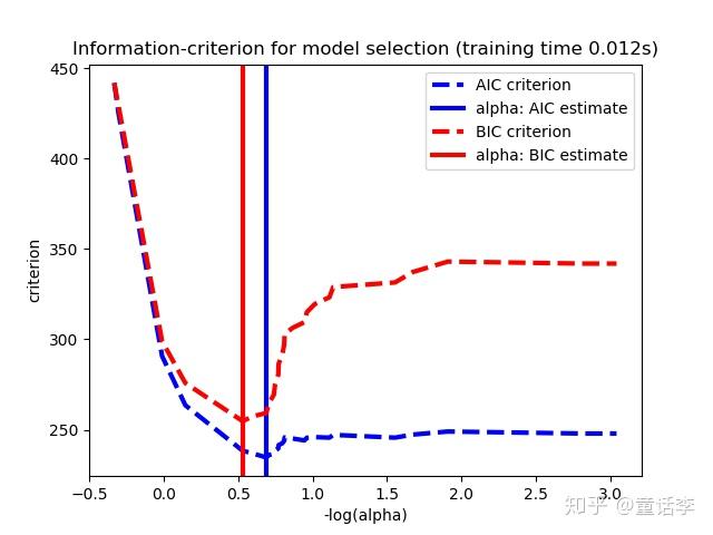
如何选择合适的$\alpha$呢?
LASSO和RIDGE一般用赤池信息准则(AIC)或贝叶斯信息准则(BIC)来选择$\alpha$,AIC大致是关于惩罚力度的U型函数,条件形同的情况下AIC越小越好,直接选取AIC最低点对应的惩罚力度$\alpha$。
总结
- Key Difference
- LASSO
- LASSO可以对特征进行选择,就像我们观察到的那样,很多系数变成了0。 - RIDGE
- 它包含所有特征。
- LASSO
- Typical Use Cases
- RIDGE
- 主要用于防止过拟合。因为它包含了所有的特征,所以在高维度的情况下(比如以百万计),它不是很有用,因为计算量太大。 - LASSO
- 因为它提供了稀疏解,所以它经常在高维度数据建模中使用。在这种情况下,得到一个稀疏解具有很大的计算优势,因为零系数的特征可以简单地忽略。
- RIDGE